This post was written as a part of my exam preparation for the course in Low Energy and Reconfigurable Systems at AAU. It is a write-up from a mini project done in cooperation with two of my fellow students. The mini project goes through an architectural design of the CORDIC algorithm for calculating the $x$ and $y$ values of a cosine, given an angle. The architecture is at the RTL level and should need no further processing before implementation. Actually, it also goes through the mathematical derivation of the CORDIC algorithm, but I won’t bore you with that. You just need to know that the algorithm uses “microrotations” to match the angle using the math below
$$x_{i+1} = x_i - \sigma_i \cdot 2^{-i} \cdot y_i$$
$$y_{i+1} = \sigma_i \cdot 2^{-i} \cdot x_i + y_i$$
$$z_{i+1} = z_i - \sigma_i \cdot arctan(2^{-i})$$
Where we set $x_0 = 1$, $y_0 = 0$ and $z_0 = \theta$. Then $\sigma_i$ becomes the sign of $z_i$. Which will then be the input of the algorithm. It should be noted that the computation $2^{-i}$ can be done by shifting the operand we are multiplying it with. Also, we are able to calculate $arctan(2^{-i})$ beforehand and store it in a table for faster computation.
The pseudo-code for the algorithm is listed below.
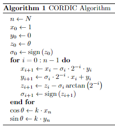
Psedo code for CORDIC algorithm
The constant $k$ is calculated as $\prod_{i} k_i = \prod_{i} \frac{1}{\sqrt{1+2^{-2i}}}$. Meaning this constant can also be calculated beforehand.
Numerical aspects (fixed vs. floating point)
We wanted to test some of the aspects related to using a fixed point algorithm. Specifically, we wanted to see how many iterations we would expect to have before the algorithm converged over the number of decimal bits used in the fixed point. This was tested in Python using the FixedPoint library. The results are shown in the figure below.
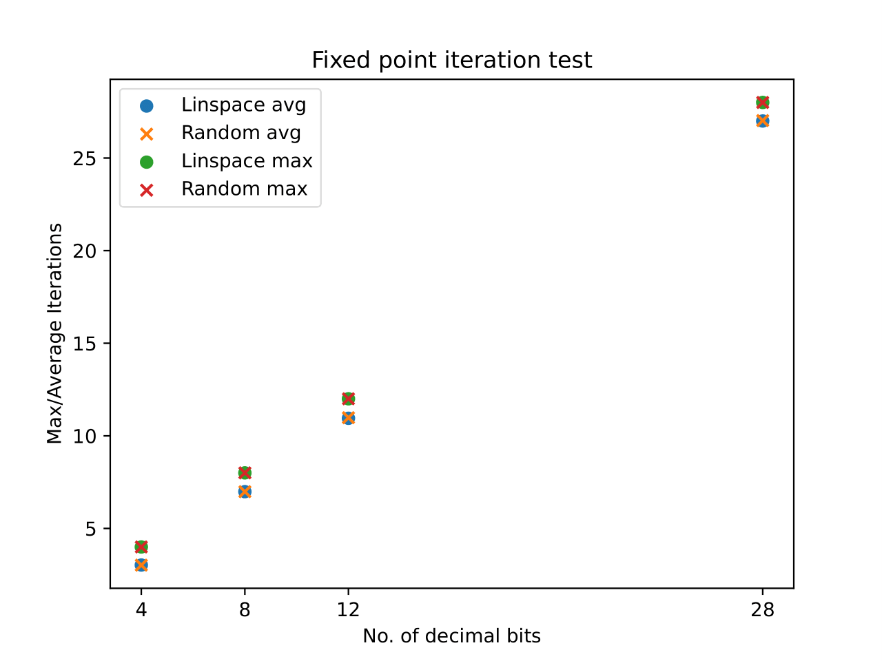
Iterations to run algorithm compared to the number of decimal points
The figure shows that if high decimal precision is required, then more iterations are needed before the algorithm converges. Which makes sense. We had an internal discussion about whether the results would change if the angles used for the input were generated randomly instead of linearly, so both are included in the figure. Next, we tested the error between the standard Python floating point precision and the algorithm output over the number of decimal bits. The results of this can be seen in the figure below

Fixed point/Floating point resulting error from different bit precisions
The figure shows that beyond $12$ decimal bits the error is more or less the same. Even $8$ decimal bits are useful. Thus based on the previous two figures, we chose a $12$-bit 2-complement implementation, with a maximum of $11$ iterations before termination. This can be described in the $Q$-number format as $Q3.12$, where we have four integer bits with MSB being the sign bit.
Graphical Representations
The hardware implementation of the algorithm could consist of a single CORDIC element, that would then be reused for each iteration. But instead, to take advantage of maximum parallelization and be able to have a continuous input, several CORDIC elements are used. So basically we are using one CORDIC element per iteration up to the maximum number of iterations. The elements will then be connected sequentially.
Synchronous Data Flow
Each element is referenced as $CE_i$ and the inputs are connected to $CE_0$ while the output comes from $CE_{10}$, as shown in the figure below.
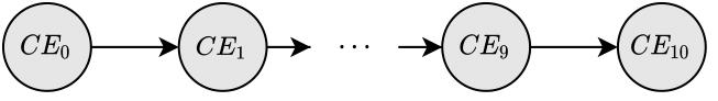
Example of a CORDIC element chain
We can then open up each element of the previous figure and create a Synchronous Data Flow Graph (SDFG). From the previous figure, we note that $CE_1$ to $CE_9$ operates in the same manner. Taking this into account, we get the following SDFG
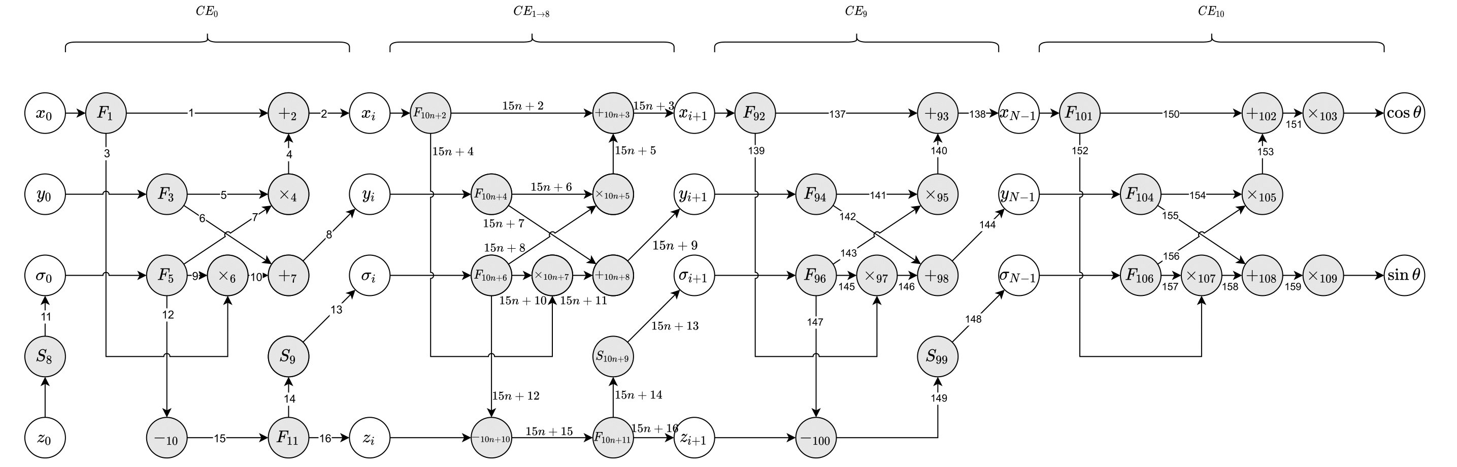
Synchronous Data Flow (SDF) graph
Nodes denoted by $F_i$ are fork nodes and do not have any arithmetic operation associated with them. Fork nodes are not considered to cause any execution delays in further system design and are only shown for readability. Nodes that are denoted by $S_i$ take the sign bit from $z_i$.
Having created these graphical representations, we can take a deeper dive into the SDFG and create the precedence graph.
Precedence Graph
The Precedence Graph (PG) also often referred to as a Dependency Graph, is used to visualize dependency between operations or tasks in the algorithm. In doing so, we are also able to determine the Critical Path (currently assuming that all operations require the same amount of time to execute). The PG can be seen in the figure below.
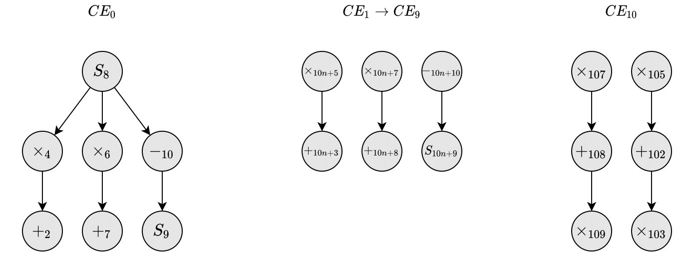
Precedence Graph
To optimize the architecture and take advantage of the parallelism of the system, we can insert a delay between all the $CE$ elements. By doing so, we make sure that the algorithm can run continuously and that all the elements can execute at the same time (still under the assumption that all elements have the same processing time from input to output). As shown in the figure below.

Chain of CORDIC elements with inserted delays
We’ve also put a limit on the number of function units that are available for multiplication and addition in each of the $CE$’s. Every $CE$ will have one shifter (for multiplication) and one adder available. We can use shifters for most of the multiplications since many of them are something multiplied with $2^{-i}$, which can be done by right shifting $i$-times. Meaning we end up with 11 shifters, 11 adders, and two multipliers for the 11-iteration CORDIC algorithm. The following scheduling section will show how this is possible.
Scheduling
We can use the previously created DFG and PG to create a schedule for the algorithm. For this, we will use the ASAP & ALAP methodology, which is where we first schedule operations as soon as possible and afterward, they are scheduled as late as possible. The methodology makes it possible to calculate the mobility and urgency for each operation, which in turn, we can use to create a prioritized ready list. ASAP and ALAP schedules can be seen in the figures below.
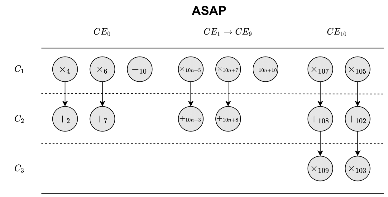
As Soon As Possible Scheduling
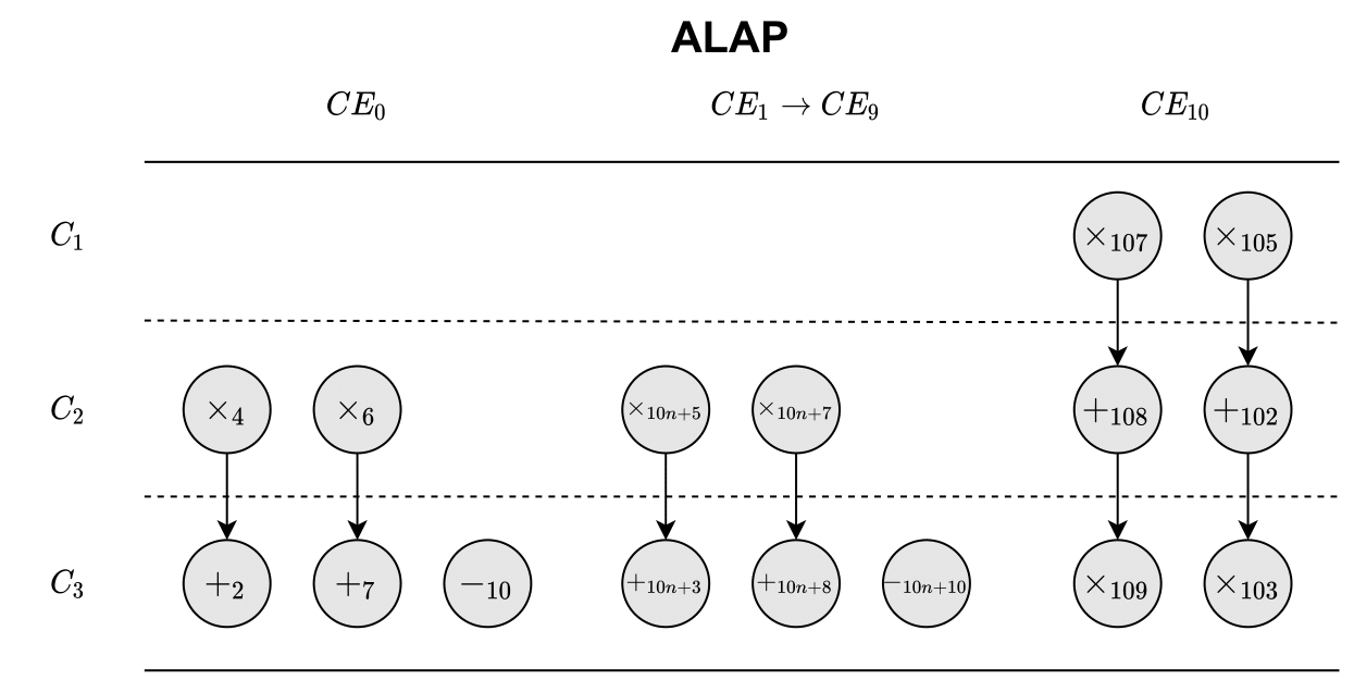
As Late As Possible Scheduling
The $C_i$’s on the left side of each plot corresponds to a C-step.
Mobilities can then be calculated using the following expression
$$M(op) = ALAP(op) - ASAP(op)$$
Where $M(op)$ is the mobility of the operation $op$. Then $ALAP(op)$ is the C-step where $op$ is scheduled in ALAP, and the same thing goes for ASAP. Below an example is shown for calculating $M(x_4)$.
$$M(x_4) = ALAP(x_4) - ASAP(x_4) = 2 - 1 = 1$$
So for $CE_10$, the mobility for all operations is zero since they are all scheduled at the same time in both schemes.
Having calculated the mobilities for all the operations, we can go on to calculate the urgencies. Which we can calculate using the following expression
$$U(op) = \frac{w}{CS}$$
Where $w$ is a weight associated with each operation that can be defined in different ways. $CS$ is the number of control steps we go through until we hit the c-step where the operation is scheduled in ALAP. For this implementation, we will set the weights equal to the computation times of the operations. But since we have assumed that all operations take the same amount of time to complete, we will set all the weights to $1$.
Operation Schedule
As we have previously already stated the allocation of our resources (i.e. one adder and one shifter per $CE$), we can now schedule from the results above. For every C-step, we can only do one shift operation and one addition in each $CE$. So for $CE_0$, the shifting operations $x_4$ and $x_6$ have the lowest mobility and the highest urgency and should be scheduled first. Because of only having one bit-shifter, we have to schedule them in two C-steps. As they also have the same mobility, we can schedule them randomly.
We will schedule $x_4$ in the first C-step and $x_6$ in the second C-step.
Now, our resource allocation also permits us to schedule an addition/subtraction in the first C-step, but since both $+_2$ and $+_7$ are dependent on $x_4$ and $x_6$ respectively, we cannot schedule those in C-step $1$.
The only operation left for scheduling then is $-_{10}$. For C-step $2$, the only addition that is available to perform is $+_2$ as $x_6$ is also scheduled for this C-step. We’ll end up scheduling $+_7$ in C-step $3$. This scheduling scheme is used for $CE_0$ to $CE_9$. For $CE_{10}$, we can see from the ASAP and ALAP schedules that the operations have no mobility, so we have to schedule them as is. Meaning we’ll end up with the following schedule.
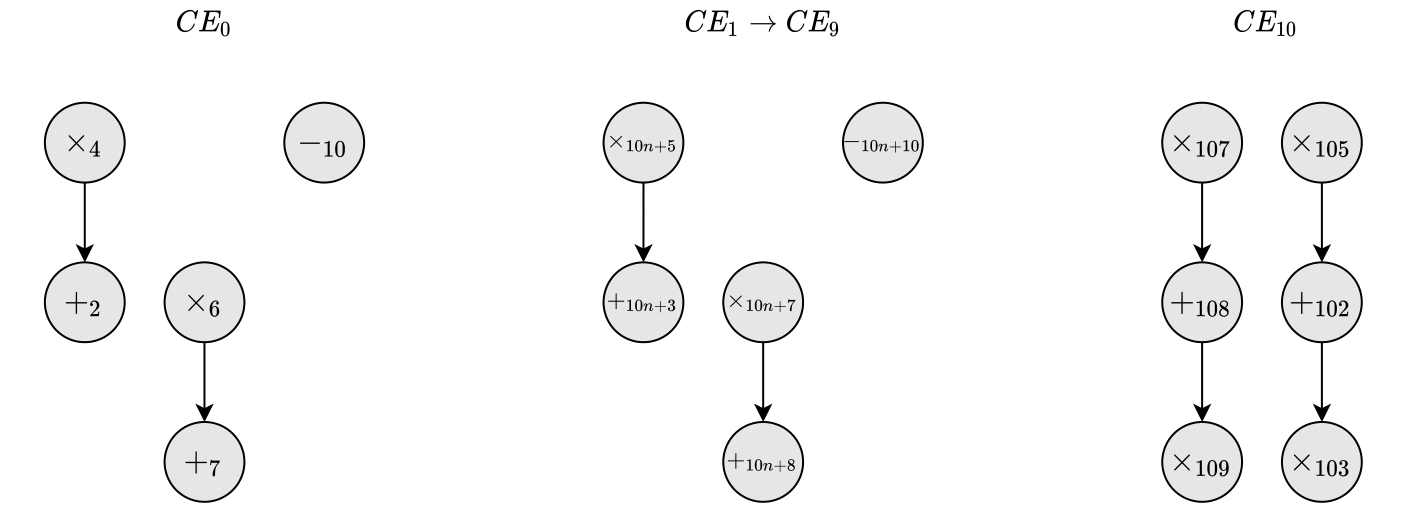
Precedence Graph according to schedule
The scheduling scheme now permits us to illustrate the system as a Finite State Machine (FSM). More specifically, we will illustrate the system as an Algorithmic State Machine (ASM) that has 3 states. Each state is defined as one of the C-steps in the schedule shown above. The ASM can be seen below.
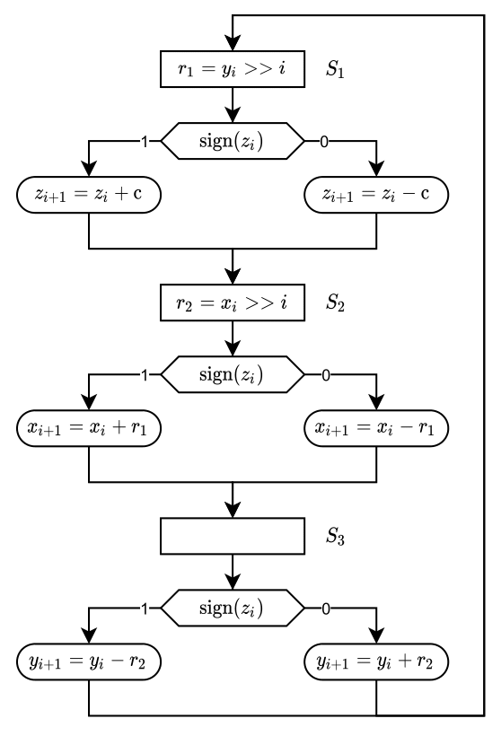
Algorithmic State Machine
From the ASM we can see that the output logic is dependent on $sign(z_i)$, which in our case is an input to each of the $CE$’s. Hence we can define the FSM as a Mealy Machine.
Datapath
The datapath of a system is a collection of the operations, registers and the connections between them. Since the system we are designing both have time-constrain considerations as well as area constraints, each of the $CE$’s will have dedicated hardware such that inputs and outputs can be run “continuously”. From the schedule, we can see that the datapath for $CE_0$ to $CE_9$ is identical.
Our, however, $CE_{10}$ does not share the same schedule and must therefore have a different datapath as there are more operations to consider. By using the schedule shown just before, we can implement the SDFG that we previously illustrated. The results are the datapath below.
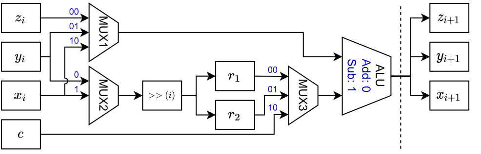
Datapath for most Cordic elements
State input/outputs are switched using multiplexers shown with bit sequence control inputs on each line. Registers are depicted by boxes. The bit-shifting operation is denoted by the square box with the operation $»(i)$, which as mentioned equivalent to shifting $i$-times to the right. Internal registers are denoted by $r_1$ and $r_2$, while registers on in/output are denoted by the respective variable names and $CE$ element count. We will write to an output register at each state, so a control signal to each of the registers is needed. Since $CE_{10}$ is different from the rest of the elements, we create a unique datapath for it, which is shown below.
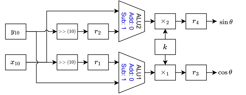
Datapath for specific Cordic element.
The datapath shows that $CE_{10}$ is used as the output element and the cosine and sine to the input angle $\theta$ is the output. We also see the two actual multipliers in the system (not the shifters as in the other elements). We also require two ALUs for this element to process both outputs in parallel.
Control Signals
We cannot rely solely on the data path. Thus, as previously shown in the CDFG, we also need a control path. Signals from the control path are connected to the datapath such that operations can be timed to the correct state. All generated control signals are shown in the table below.
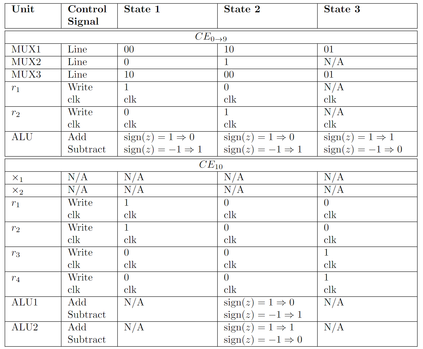
Table of control signals.
Multiplexers that can control more than one input will be controlled by two-bit signals whereas we can control two-input multiplexers with only a one-bit signal. Each register will have a control signal such that it can be read from or written to. Further, ALUs will have a control signal such that we can switch between addition and subtraction, based on $sign(z)$.
RTL Design
Having defined a datapath, ASM and a schedule, we can start thinking about implementing the algorithm in Register Transfer Level (RTL). We have chosen not to explore the actual implementations of adders and multipliers, which means we only use IP blocks from the Quartus library.
Multiplexers have been implemented as two different functional units with different amounts of input and control signal input sizes. The RTL diagram can be seen in the figure below.

RTL illustration of the internals of a Cordic element.
The RTL follows the datapath closely and the only difference in the two diagrams is that control signals are also shown in the former. The bit shifter in each of the $CE$ elements needs to know how many times to shift. Therefore a constant has been defined for each of the $CE$s. This constant is hard coded and is therefore not part of the control flow. Now we need to put multiple $CE$s together which can be seen in the RTL diagram below.
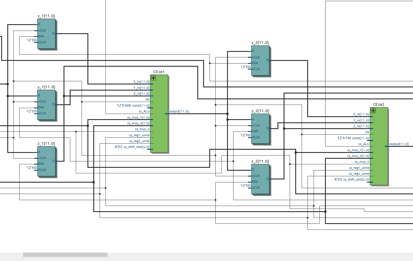
RTL illustration showing the connections between two Cordic elements.
Control Unit
Control signals are implemented in a separate block and can be seen in the figure below.
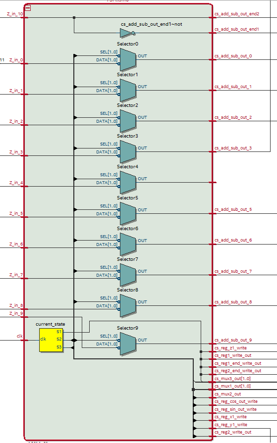
RTL diagram of the control signals and FSM
The FSM is implemented as the yellow box in the diagram and contains state information about the current and next state. The output of the FSM is connected to a bus that also connects to a bunch of multiplexers. In this way, the control signals can be switched to match the current state operations. There are still some bugs in the implementation which we have not been able to fix yet.